What if we could only draw straight lines on a canvas? Could we be able to create art under such a constraint?

A few weeks ago, I came across a very talented artist, Petros Vrellis, who created interesting art pieces by only using straight lines. Several others have tried to recreate this type of work, such as Christian Siegel and Shlonkin.

I have been curious about understanding the underlying dynamics that work with this constraint. Therefore, in this post I implement an algorithm where given an image, it creates a new image by only drawing straight lines. Here, I perform an in-depth analysis on the parameters that can be tweaked for this algorithm to work.

SAMPLE IMAGE

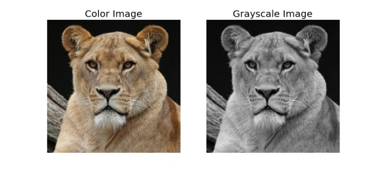
As we develop the algorithm, we require a sample image to test. I selected a photograph of a lioness, which is presented below as both a color and grayscale image. The image was cropped so that it has a square shape; however, the algorithm works as well on rectangular images.

The goal of the algorithm is to recreate the grayscale image (GI) by drawing straight black lines on a white background (or straight white lines on a black background). In this study, we describe the algorithm that draws black lines on a white background; however, the opposite can be implemented by flipping the black and white values. The new image will be referred to as a Line Image (LI).

Here is a video that shows an example of how the algorithm works:

ALGORITHM

The algorithm is described below:

Select a Start Point on the border of the image.
Select an End Point on the border of the image.
Find the Mean Pixel Intensity (MPI) for a straight line between the Start and End Points. The value of a grayscale pixel is an integer between 0 (black) and 255 (white).
Repeat steps (2) and (3) for all possible Start and End Points.
Select the line which contains the lowest MPI.
Subtract a line with a specific grayscale level from the LI. If at some point the value of a pixel goes below 0, truncate it to 0.
Add a line with a specific grayscale level from the GI. If at some point the value of a pixel goes above 255, truncate it to 255.
Repeat from step (1) until the whole image is drawn.

STARTING POINTS

The starting point of each line can have one of three possible options:

Previous Line End-Point: in this case once a line is drawn from point A to B, the next line is drawn from point B to C. In other words, the ending point of the previous line is the starting point of the next line.
Random: we select randomly the start point of every line.
Optimum: we look at all possible start-end pairs and find the one that has the lowest MPI .

The Optimum start point is ideal; however, it is the most computational intensive, given that we calculate the MPI for all Start-End Point combinations. However, the Random and Previous Line End-Point are bound by the Start Point and only needs to compute the MPI for all possible End Points. In this study, we analyze the Previous Line End-Point case.

PARAMETERS

As we work on implementing the algorithm we have three main parameters that are defined below:

Number of Lines to Draw
Grayscale Levels
Number of Pegs (Pixels Between Pegs)

Number of Lines to Draw

To determine the optimum number of lines to draw we need an exit criteria for the algorithm. I opted to minimize a cost function; specifically, the least squared error between the original GI and the LI. The equation is:

where L is the number of lines, N is the total number of pixels in the image, and I is the image. We select the L that minimizes LSE(L). In this equation, we normalize the error by a factor so that the LSE values are not too large.

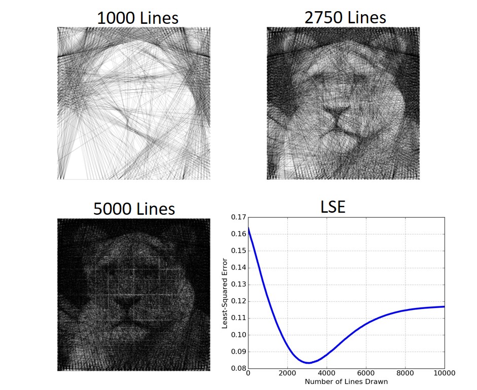
Below we present examples of the image drawn with different number of lines. The LSE as a function of number of lines drawn is also presented. We can observe a few key elements. First the LSE decreases as the number of lines increases, until it reaches a minimum which is the optimum solution. In this case the minimum LSE occurs at 2750 lines. After that the LSE increases but eventually reaches a saturation point. The saturation point occurs when the LI is black; therefore, adding more lines does not alter the LI.

Grayscale Levels

Each pixel on a grayscale image can have an integer value between 0 (black) and 255 (white). When we add a grayscale line to the LI or remove the grayscale line from the GI, the pixels in the line can have a value between 0 and 255. For example, we can have 1 grayscale level meaning that we add a line with a grayscale value of 255 to the LI. If we have 2 grayscale levels, we add a line with a grayscale value of 128. And so on.

In the image below we present the results for 1, 2, 3, 4 and 8 levels of grayscale. We also present the LSE calculated at the optimum number of lines for each case. We observe that the more grayscale levels produce the smallest LSE, which can be perceived in the finer details of the LI. Similarly, we show the optimum number of lines required to be drawn. The higher the number of grayscale levels requires a higher number of lines to be drawn.

Number of Pegs (Pixels Between Pegs)

The peg is defined as the anchor points at the border of the image where the lines will start/stop. For a given image resolution we can define the Number of Pegs (#Pegs), and the number of Pixels Between Pegs (PBP). The equation that defines this is given by:

where the #Pix is the number of pixels on 1 of the axis of the image. For example, in the lioness image, the resolution is 981x981 pixels. Below is a table that shows the number of pegs and pixels between pegs we used to test the image.

Below we show the images resulting by using different number of pegs per side, as well as the LSE obtained at the optimum number of lines. The higher number of pegs (lower number of pixels per peg) produces the image with the highest resolution. Similarly, the higher the number of pegs, the more number of lines is required.

CONCLUSIONS

In this post, we demonstrated an algorithm that can convert any grayscale image into an image drawn with lines. We establish that there are 3 parameters that affect the image. There is an optimum number of lines that need to be drawn which minimizes the cost function. Similarly, the higher the number of grayscale levels and the higher the number of pegs, the better the quality of the output image. However, the drawback is that the algorithm requires more computational time, when the parameters are optimized. Therefore, a balance needs to be selected between the run-time of the algorithm and the quality of the image. If we select high quality parameters such as 8 grayscale levels, and 99 pegs (10 pixels between pegs), we can obtain a high-quality image, such as the one shown below (7050 lines with an LSE = 0.055).

Another application of this algorithm is to create videos where each frame is a LI. Below we present an example of a 4 second video of a puppy.

Finally, it is important to mention that others have created variations of this form of art such as Linify, and vector graphic images.