One of the challenges in building models is mixing features that have different scales. For example, we may want to predict somebody's risk for diabetes using, among other things, their height and weight. The height may have units of feet with a range between 0 and 9, and the weight may have units of lbs with a range between 0 and 1000. When we mix units with ranges that have different orders of magnitude, our models may not be able to find the proper coefficients.
In the previous post, we demonstrated that by normalizing the features used in a model (such as Linear Regression), we can more accurately obtain the optimum coefficients that allow the model to best fit the data. In this post we will go deeper to analyze how a method commonly used to extract the optimum coefficients, known as Gradient Descent (GD), is affected by the normalization of the features.
We will use data with the following linear model:
In this case we are trying to obtain the best β's that will minimize a cost function J which is defined as the mean squared error (MSE).
DATA SET
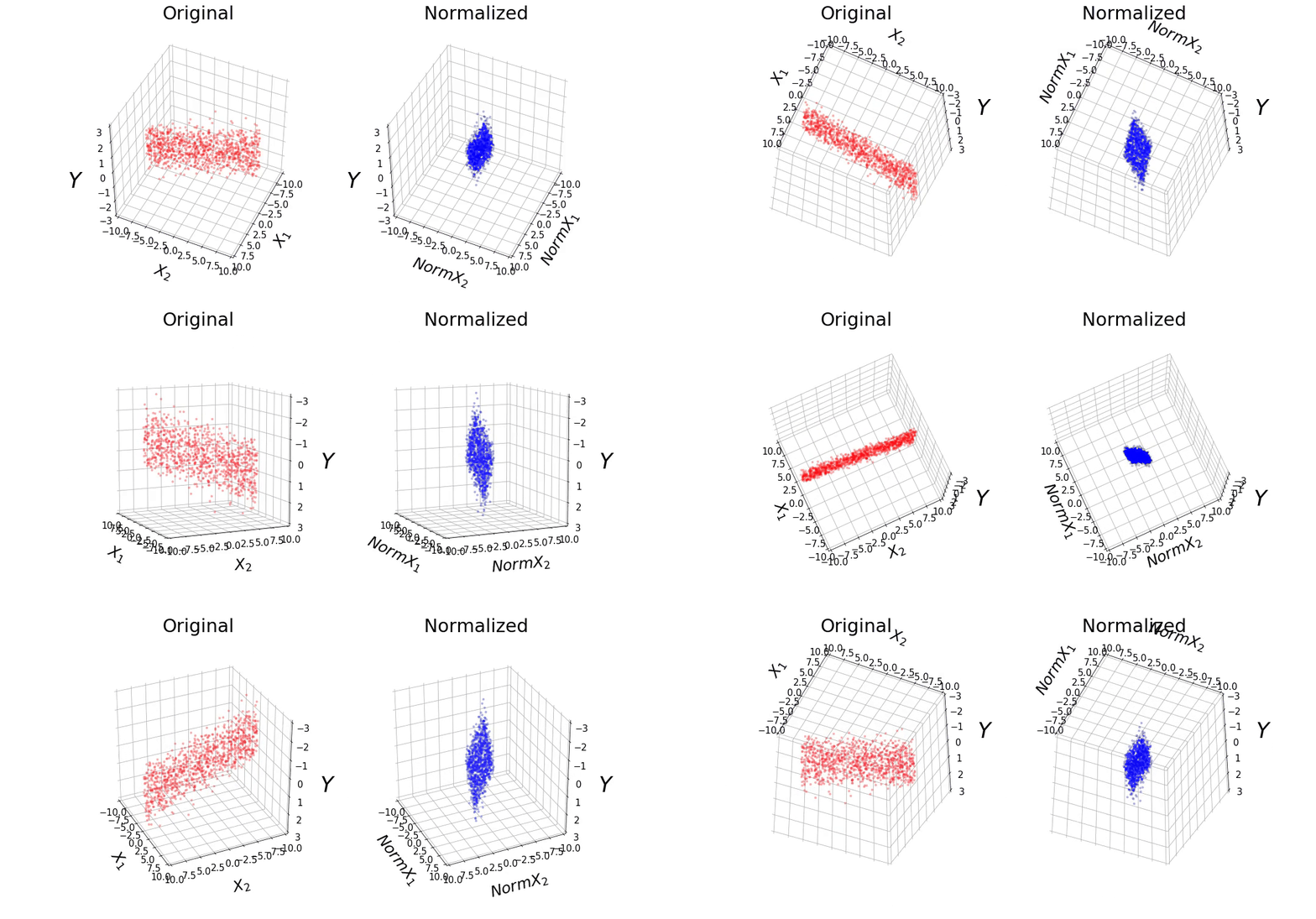
The data consists of 1,000 points randomly selected from a uniform distribution. We will make the ranges of the features vary between -0.1 and 0.1 for X1, and -10 and 10 for X2. We will also define β1 and β2 as 10 and 0.1, respectively. It can be observed that the range of the features differ by 2 orders of magnitude. We also added Gaussian noise to the target variable (y) with a mean of 0 and variance of 0.5. This data set will be referred to as the "Original" data.
We also normalized the features, such that it has a mean of 0 and a variance of 1. This data set will be referred to as the "Normalized" data. The data from the "Original" and "Normalized" set can be observed below. Although the features have different ranges between both data sets, they have the same values for y.
Figure 1: (A) Original and (B) Normalized data.
GRADIENT DESCENT (GD)
Gradient descent is an algorithm commonly used to find the optimum parameters without using an analytical solution. Although it is possible to use linear algebra to obtain the coefficient of the β's using the following equation:
it is computationally expensive to make it work when the number of features and/or data points is large. Therefore, iterative algorithms such as GD can come in handy.
The explanation of GD is beyond the scope of this post, and further details can be found here. However, the idea of GD consists of selecting at random the value of the β's, and calculating the cost function at that point. Given that the MSE is differentiable and convex (this is important because it means it only has 1 local minimum which is also the global minimum), we can determine its gradients and take a step in the opposite direction of the maximum value (direction where the slope is the steepest). The size of the step will be given by the product of a parameter known as the learning rate (α) times the gradient. The step size will be larger as the slope is steeper. The β's get updated using the following equation:
LEARNING RATE
There are two parameters that need to be defined when we run GD, the starting point of the coefficients, and the learning rate. In this section we discuss the latter. We will run GD on both the "Original" and "Normalized" data set while using different learning rates. We expect that when the learning rate is small, it will take several steps to converge. On the other hand, when the learning rate is large, it may never converge (it diverges) because the step size is too big, and it always overshoots the optimum values for the feature coefficients. The learning rate that reaches the minimum of the cost function with the least amount of steps would be the optimum. In this case, we will initialize the feature coefficients to -10, for both of them, and we will try several learning rates between 0.025 and 0.075.
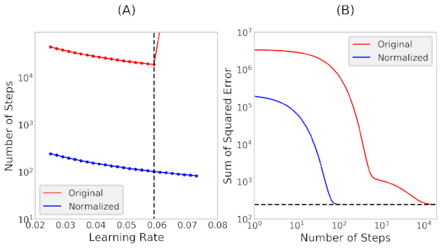
Figure 2: (A) Number of steps taken as a function of the learning rate. (b) Sum of squared error as a function of the number of steps taken.
It takes the "Original" data set about 100X more steps than the "Normalized" data set to reach the optimum coefficients, as observed in figure (A) above. It can also be observed that for the "Original" data set, the cost function has a minimum at a learning rate of 0.059, indicating that this is the optimum learning rate. On the other hand, the "Normalized" data set, did not reach the minimum of the number of steps with the learning rates tested. Although we could still use a larger learning rate in the "Normalized" set, for the rest of the analysis we will use the learning rate of 0.059 for both data sets.
In figure (B) we present the cost function versus the number of steps taken when the learning rate is 0.059. We note that the "Normalized" data reaches the minimum cost function in 100x fewer steps than the "Original" data set.
The image below presents the number of steps required to find the optimum β's. The x-axis presents the number of steps and the y-axis is the value of the β. In figure (A) we observe that the "Original" data requires about 10,000 steps for β1 to reach its optimum value (black dashed line). Also, it starts adjusting its value after β2 reaches its optimum as observed in figure (C). We notice that for β2, the number of steps required is about 100, but there are big oscillations on selecting the optimum value. We can summarize this by indicating that the learning rate is too small for β1 (taking a long time to converge), and too large for β2 (oscillating several times before converging). If the learning rate is increased, it would diverge and never reach its optimum point.
On the other hand, we notice that when the data is "Normalized", it takes about 100 steps for the β's to converge, figures (B) and (D). Both β's converge simultaneously. The learning rate here could be increased more to minimize the number of steps required.
Figure 3: Number of steps to reach β1 and β2 for the "Original" and "Normalized" data sets.
BETA PATHS
To obtain a better intuition about how the GD algorithm updates the β's, we can create a plot that shows the path taken through the cost function. In the image below we present a heat map, where the color indicates the cost function at different β's. The x-axis presents β1 and the y-axis β2. The goal is that we start at a point (-10,-10) indicated by a red dot, and thru GD we want to take steps to reach the minimum of the cost function, indicated by the red "X". The orange line shows the path taken by the GD algorithm. We note that for the "Original" data set, shown in figure (A) below, the GD algorithm quickly finds the value for β2, and then it adjusts to find the value of β1. Generally speaking, the path was mostly in the vertical direction first, and then in the horizontal direction. When we observe the "Normalized" version, shown in figure (B) below, we notice that cost function follows a circular shape. The path followed is a straight line, which is the shortest distance between the starting and ending points
Figure 4: Path thru the cost function of the gradient descent algorithm for the (A) Original and (B) Normalized data sets.
STARTING POINT
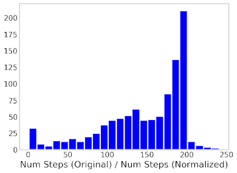
We previously mentioned that for GD we specify two parameters, the learning rate and the starting points. In the previous analysis, we focused on using a fixed starting point of (-10,-10). What happens if we use other starting points? We ran the GD using 1000 different starting points within the ranges of -20 and 20, and determine how many steps are required for the GD to converge. We took the ratio of the number of steps taken in the "Original" over the "Normalized", and created a histogram presented below. Note, that if the starting points are very close to the true β values for the "Original" data set, these may converge quicker than the "Normalized".
Figure 5: Histogram of the Ratio of the Number of Steps taken between the Original and Normalized dataset.
From the image above we learn that the "Normalized" data set tends to require less number of steps to reach the .minimum of the cost function, compared to the "Original" data set.
CONCLUSION
Thru the last two post, we have been able to understand the influence of normalizing the data when using techniques such as GD to obtain optimum values of the β coefficients. In summary, one should always "Normalize" the features to be able to speed up convergence. The code can be found here.


